Notes on simple linear regression and 2D point clouds
Linear regression is to statistics what Wonderwall is to guitar : you learn it at the very beginning, it looks simple and naive, and after you saw it once you don’t really want to hear about it again. But surprisingly it hides a lot of subtleties that I keep discovering years about seeing my first linear regression. In particular, after thinking about its links with PCA and correlation I found some very simple and elegant relationships that I want to share in this post. This is the story of why linear regression is both more complicated and more simple than what you thought.
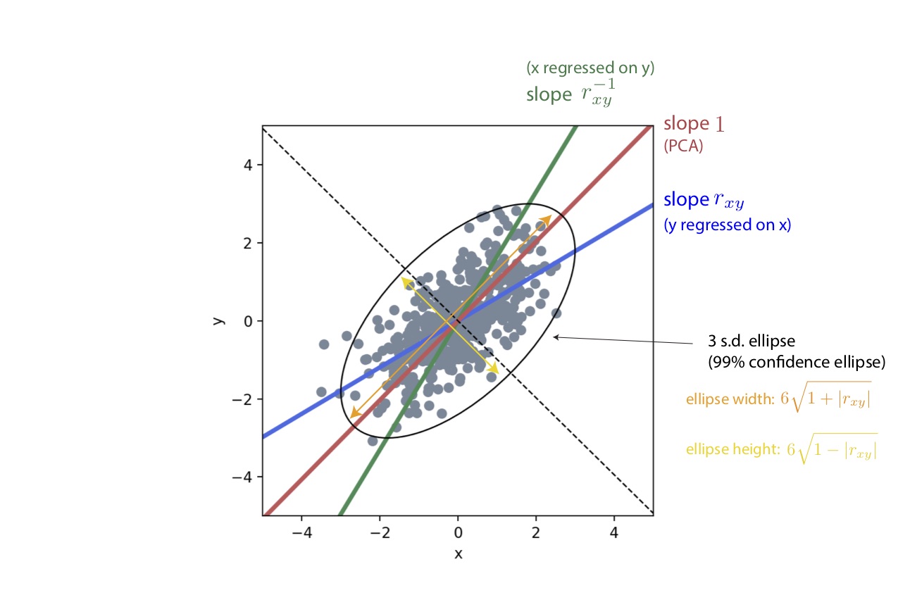
Figure 1 : Too long, don't wanna read the post ? Pretty much everything is here (for centered, standardized data)
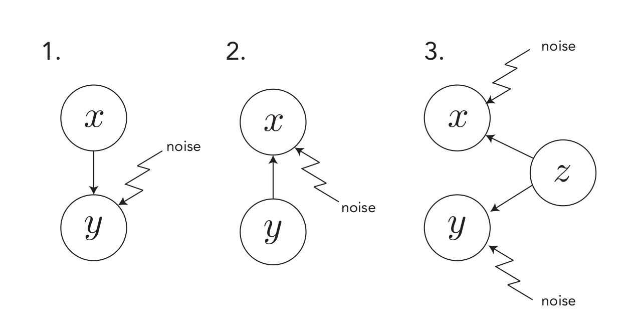
Figure 2 : the three types of causal models seen here.
Disclaimer: I have the derivations for all that’s written here. At some point I might find the time to add them in an appendix to the post.
The three fitting lines.
Given a two-dimensional cloud of points, one can choose to fit several lines to it. Let us consider some data $({(x_i, y_i)}_{1 \leq i \leq n}$. We will assume it is centered, ie. $\sum x_i = 0 = \sum y_i$ without loss of generality. Sometimes I will assume standardized data (ie. such that $\operatorname{Var}[x] = \operatorname{Var}[y] = 1$) which gives more elegant formulas but will mark all formulas that hold only in this case in blue to avoid confusion.
One could wish to predict $y$ from $x$, thus performing a linear regression of $y$ onto $x$. This corresponds to fitting the $\beta_0$ parameter in the model :
where $\epsilon \sim \mathcal{N}(0, \sigma^2)$ while minimizing the error variance $\sigma^2$. This corresponds to a causal model where the target variable $y$ is generated by fixed values of $x$ and a source of noise (see figure 2). This gives the classical linear regression model, whose solution is given by :
where $\sigma_x$ and $\sigma_y$ are the standard deviations of $x$ and $y$ (the square root of their variances) and $r_{xy}$ is the Pearson correlation coefficient between $x$ and $y$, given in general by :
And if the data is moreover standardized, this gives the very simple relationship :
Alternatively, one could want to consider the inverse prediction problem : predicting $x$ from $y$, with the model :
Naively one could think “well, if $y \approx \beta_0 x$, then surely $x \approx \beta_0^{-1} y$ and we can simply take $\tilde{\beta} = \beta_0^{-1}$ ?”. Ayayay, nothing could be more wrong ! To understand this, consider the simple example where $\beta = 0$, which leads to $y = \epsilon$. In this situation, $x$ and $y$ are actually two independent random variables, so we can also say that $x$ does not depend on $y$ and conclude that $\tilde{\beta} = 0$ too. Actually, just as above we can write the optimal solution for $\hat{\tilde{\beta}}$ as:
I am going to inverse it so that we can plot it while still having $x$ on the abscissa and $y$ on the ordinate so that we obtain our second fitting line with slope :
And we note that if the data is standardized we get:
In this case we see that we obtain two different lines fitted to the same cloud of points and symmetric one of the other with the respect to the central diagonal $y=x$ (or $y=-x$ if our correlations and slopes are negative). Which means that… in the end, what is the best fitting line to our cloud of points ? Is any line in between those two also valid ?
Actually, let us get rid of the causal models whereby $x$ generates $y$ or the opposite. After all, “data is all there is to science” as Judea Pearl says. A third idea could be to perform a PCA on our cloud of points and consider its first component as the line that explains our data the best. We can derive this first component particularly in the case of standardized data (for non-standardized data simply multiply by $\sigma_y/\sigma_x$) and obtain:
Yes, amazingly, once we have standardized the data, one of the best fitting line turns out to simply be a slope ±1. Then what is this linear regression all about ? What information do we get in the end when fitting a line ?
Note how the three lines here are all optimal in a different way : the first one minimizes the distance from each point to the line along the y axis, the second one minimizes the distance from each point to the line along the x axis, and the last one minimizes the distance from each point to the line orthogonally to the line (the real “distance to the line” according to mathematicians).
The coefficient of determination.
I mentioned earlier the coefficient of determination, usually noted $r^2$. It is a number between 0 and 1 indicating how accurate the linear regression is, and usually magically given by linear regression routines. It is often explained as the “proportion of variance explained by the model”, which mathematically would be, if we take our first model (caution with this relation, for linear regression it appears that noise variance + model variance = Var[y] but won’t necessarily be the case for other types of models):
From this we obtain immediately:
So the notation used for this coefficient is of course no coincidence ! We find again Pearson’s correlation coefficient hidden behind it ! Actually a more general result is that for multivariate regression with several explanatory variables $\mathbf{x_i} = (x_{1, i}, \dots, x_{i, d})^T$ and one single target variable $y$, when the model $y = \boldsymbol{\beta}^T\mathbf{x} + \epsilon$ is fit, its coefficient of determination is the square of the Pearson correlation coefficient of $y$ and $\hat{y} = \hat{\boldsymbol{\beta}}^T\mathbf{x}$.
Note that we would obtain the same $r^2$ when trying to predict $x$ from $y$ instead. Now everything comes back together : the fact that we obtained two very different lines earlier was a manifestation of the fact that a linear model was rather imprecise for our data. What a linear regression does is assess how close the data can be to a line, and this is a question that is actually answered by the correlation coefficient $r_{xy}$. So in the end, the slope of a simple linear regression, when stripped out of its scaling component $\sigma_y/\sigma_x$ simply indicates its own goodness of fit, which I find to be an amazing phenomenon.
The PCA ellipse.
Before going further, I wanted to add a few words on PCA. First, what problem does it solve, and how to relate it to the data generation process of $y$ and $x$ ? You may have heard that PCA solves the problem of finding a low-dimensional (here 1D) subspace that best explains our data. There are several ways to formalize it (see (Udell 2014), appendix A p.98). PCA actually optimizes the following latent variable problem:
where $z \sim \mathcal{N}(0, 1)$ and $\begin{pmatrix}\epsilon_1 \ \epsilon_2\end{pmatrix} \sim \mathcal{N}(0, \sigma^2\mathbf{Id})$. (Note that if we assume the noise terms can have correlations and a general covariance matrix $\Psi$ instead of $\sigma^2\mathbf{Id}$ then we obtain factor analysis instead of PCA. More on this in (Tipping & Bishop 1999)) In other words, it assumes that $x$ and $y$ are both generated by a common latent $z$ via two independent noisy processes.
Now, a note on fitting an ellipse to our data. As stated in appendix B, PCA works by performing an eigendecomposition of the covariance $\mathbf{X}^T\mathbf{X}$ of our data matrix (which I note $\mathbf{X}$, but whose rows are actually $(x_i, y_i)$ so that it encompasses the 2D data). The empirical covariance $\mathbf{X}^T\mathbf{X}$ is what one would use to fit a bivariate normal distribution to the data (this distribution would have $(0, 0)$ mean because our data is centered, and that matrix as covariance). An intuitive way to visualize multivariate gaussian distributions is via their isoprobabilistic curves which happen to be ellipses (sometimes called confidence ellipses or standard deviation ellipses). The major and minor axis of these ellipses align with the first and second principal component of the data (which are eigenvectors of $\mathbf{X}^T\mathbf{X}$), and we find after derivations that its widths and heights are for standardized data factors of $2\sqrt{1 + |r_{xy}|}$ and $2\sqrt{1 - |r_{xy}|}$ respectively.
From this result, one could conclude that the proportion of error variance (as the variance on the minor axis divided by the variance on the major axis) is
Another interesting measure of dispersion used in PCA is the proportion of variance explained by the first component. This would be:
Anyway, it is again Pearson’s correlation coefficient hiding itself there !
The conclusion is that the correlation coefficient is everywhere, and that simple linear regression turned out to be a little more complex than we thought, but only to turn out to be even simpler in the end.