Low-rank RNNs in ten minutes
This post is an attempt at summarizing results obtained over five years of research in the laboratory of Srdjan Ostojic, at ENS Paris, on the uses of low-rank RNNs, in a ten-minutes read. Let’s see if that’s enough to catch your interest!
This post has been written with invaluable inputs from several lab members, in particular Friedrich Schuessler, Francesca Mastrogiuseppe and Srdjan Ostojic. Many thanks to them!
Why low-rank RNNs?
Artificial neural networks are super cool. They are known for all sorts of computational prowesses, and they also happen to model brain processes quite well. Among artificial neural networks, there are recurrent neural networks (RNNs), which contain a pool of interconnected neurons, whose activity evolves over time. These networks can be trained to perform all sorts of cognitive tasks, and they exhibit activity patterns that are quite similar to what is observed in many brain areas!
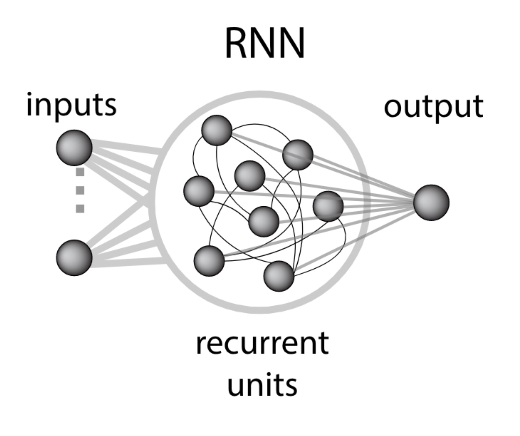
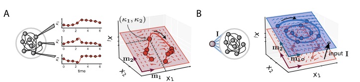
A recurrent neural network is a population of recurrently connected neurons, receiving external inputs and outputting a certain readout (from Beiran et al. 2021b).
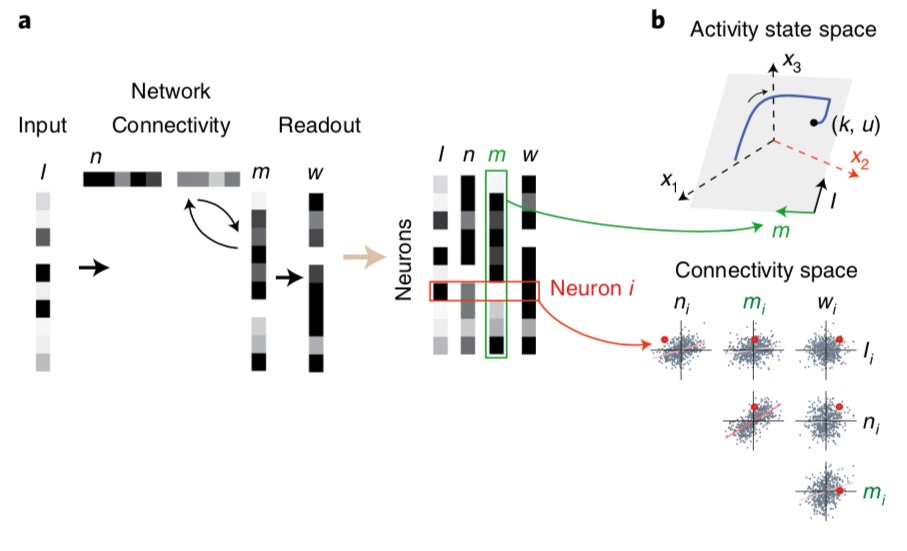
A common approach nowadays to understand neural computations is the state-space approach: one looks at the collective activity of many neurons in a network as a vector $(x_1(t), \dots, x_N(t))$ in a high-dimensional state-space. It turns out the neural trajectories in this state-space are not random, but stay confined to some particular low-dimensional subspaces, or manifolds. If you are not familiar with these concepts, a lot of places on the internet summarize them very well1. However, a big remaining mystery is how connections in a network of neurons are able to generate this very organized collective activity, able to solve complex tasks. Indeed, computer scientists have figured out how to train neural connections to get a network to do a certain task, but this doesn’t provide a deep understanding of why the obtained connections implement the task, leading some people to coin RNNs as “black-box models”.
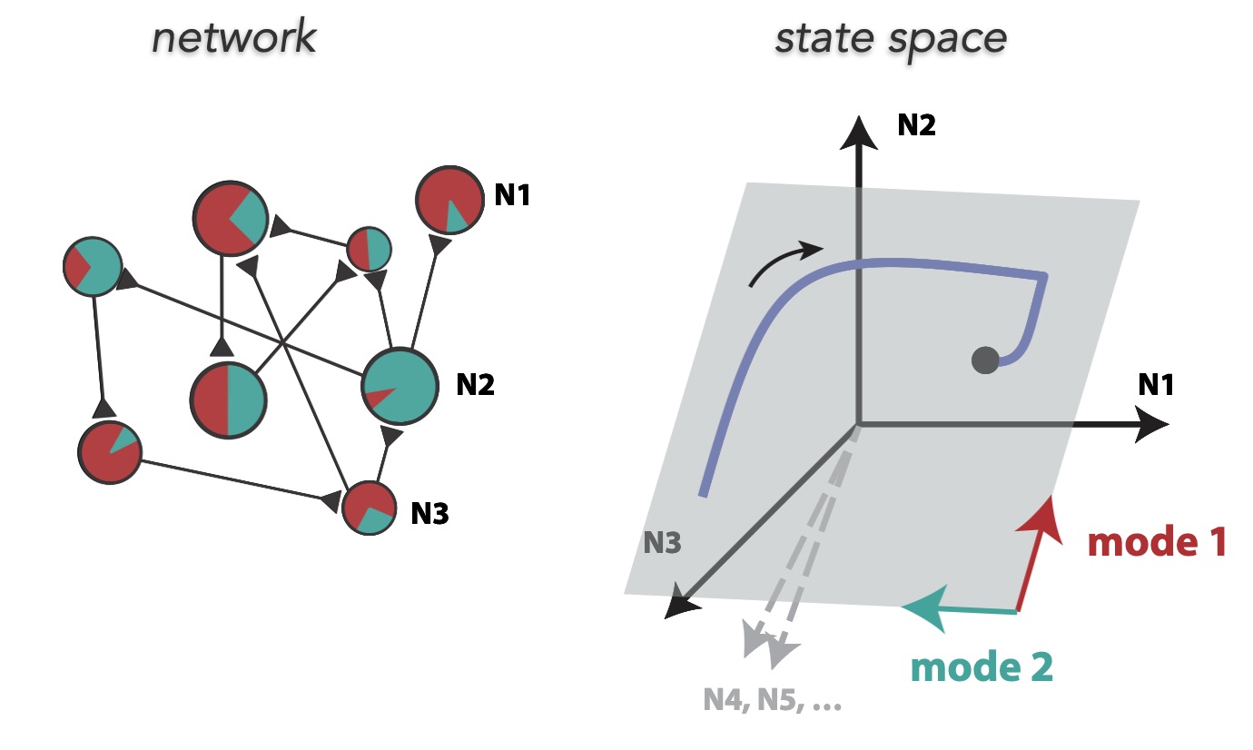
Neural state-space: each axis represents one neuron's activity or firing rate (it has much more than 3 dimensions of course). Illustration inspired on (Gallego, J. A., Perich, M. G., Miller, L. E., & Solla, S. A. (2017). Neural manifolds for the control of movement. Neuron, 94(5), 978-984.).
A first paper, published by Francesca Matrogiuseppe and Srdjan Ostojic in 20182, has shown that low-rank RNNs could be a solution to the mystery. A low-rank RNN is a network whose connections obey particular algebraic properties, namely the connectivity matrix is low-rank, and can be written formally as follows:
where $\boldsymbol{m}^{(1)}, \dots, \boldsymbol{m}^{(R)}$ and $\boldsymbol{n}^{(1)}, \dots, \boldsymbol{n}^{(R)}$, all $N$-dimensional, and $R$ is the rank of the matrix $\boldsymbol{J}$. Such a decomposition may look cumbersome, but it actually has a lot of advantages. Indeed, although they were not a general subject of study before, low-rank matrices had made many appearances in the history of computational neuroscience and machine learning, and that is no coincidence3.
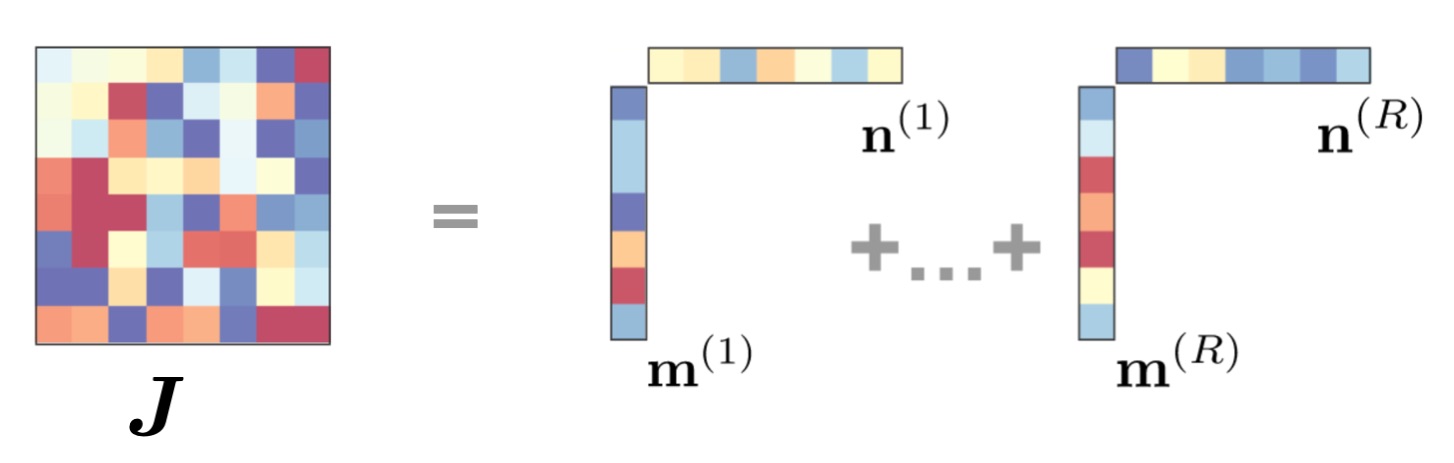
A low-rank matrix can be written as a sum of outer products of vectors. From (Beiran et al., 2021b)
In their paper, Francesca and Srdjan show that low-rank RNNs have provably low-dimensional patterns of activity, and that they can be designed to accomplish many interesting tasks like Go-NoGo or stimulus detection. An extensive mean-field theory showed that the statistics of connectivity could be linked to the dynamics of the network, paving the way for a deeper understanding of neural computations. Many papers followed, deepening different aspects of that theory, and it is now a good time to wrap up what we know about them, and what they can bring to neuroscience. I will cover some interesting tidbits about low-rank RNNs in a first part, and then give a quick overview of what the different papers are about.
Some properties of low-rank RNNs
-
Low-dimensional dynamics
Low-rank RNNs are defined in terms of vectors. There are the recurrent connectivity vectors, namely the $\boldsymbol{m}^{(r)}$ and the $\boldsymbol{n}^{(r)}$ we mentioned before, and also some input vectors $\boldsymbol{I}^{(s)}$ feeding external signals to the RNN. An essential property, easy to prove mathematically, is that the neural activity vector $\boldsymbol{x}(t)$ in a low-rank RNN is constrained to lie in subspace spanned by the $\boldsymbol{m}^{(r)}$ vectors and by the $\boldsymbol{I}^{(s)}$ vectors. We can decompose this space into a recurrently-driven subspace and an input-driven subspace, which together explain all of the activity in an RNN.
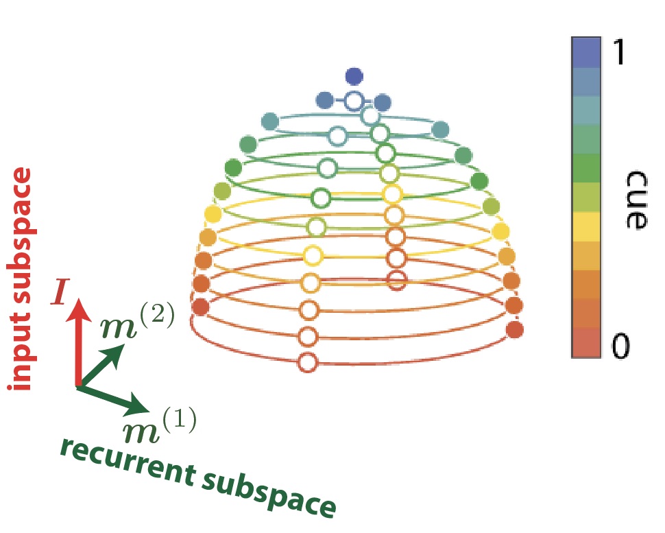
Input and recurrent subspaces for a rank-two network (hence the 2d recurrent subspace) receiving one external input. The trajectories for different input signal strengths are shown in different colors in this 3d subspace of the activity state-space. Adapted from (Beiran et al. 2021b).
In particular, when the network is not receiving any external inputs, hence generating spontaneous activity, it forms an $R$-dimensional dynamical system. If the network happens to be of rank 1 or 2, the whole set of possible dynamics can actually be visualized through a phase portrait, in which the direction and velocity of the dynamics are plotted at every point of the recurrent subspace as an arrow. Here are some example phase portraits, for a bistable network, a network implementing an oscillatory cycle, and a network implementing a ring attractor.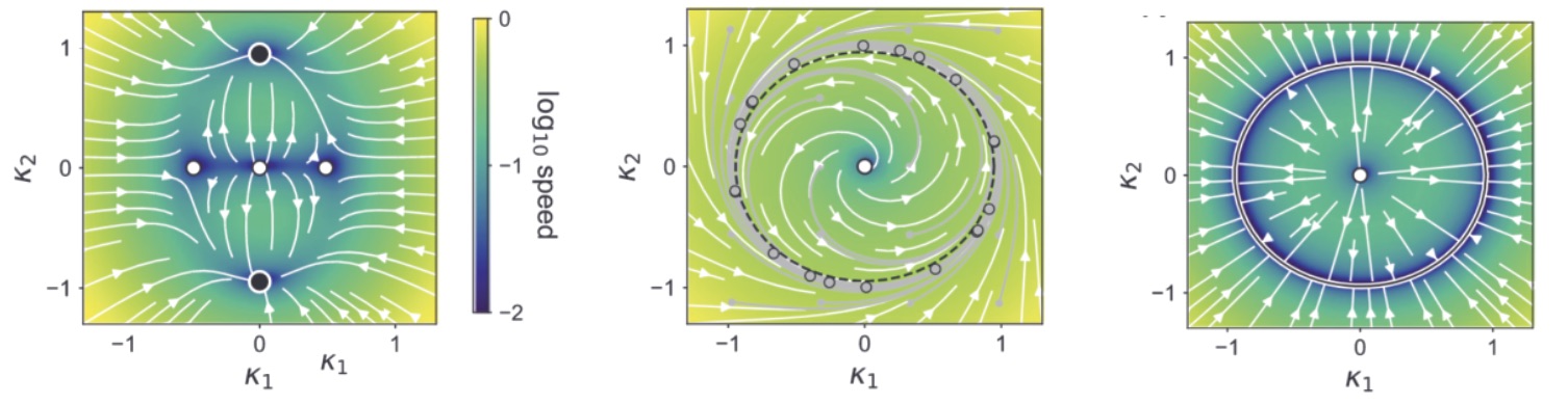
Phase portraits for three example rank-two networks, with bistable dynamics (left), a limit cycle (middle) and a ring attractor (right). From (Beiran et al. 2021a).Even for networks of rank 3, dynamics can be usefully visualized although it requires more creativity. Now what happens if we add inputs? It turns out that tonic inputs (meaning input signals that stay at a constant value for periods of time) simply move the whole recurrent subspace along an input axis towards a new region of the state-space, like an elevator, transforming the dynamics by the same occasion:
(A) illustrates how the dynamics in the absence of inputs lie in a low-dimensional recurrent subspace. (B) illustrates that in the presence of a tonic input the recurrent subspace is shifted along an input direction. Dynamics then lie on an affine subspace, and can be totally different from what they were without the input.Thanks to this property, we can still visualize the dynamics in a same network when it is receiving different inputs, and observe how these inputs modify its activity patterns. This explains how external cues could act as contextual modulators on a network, accelerating or slowing its dynamics, turning on and off certain attractors, or changing its behavior altogether.
-
The connectivity space, and the role of correlations
We have seen how low-rank RNNs can give a very visual, geometrical understanding of neural activity, but it still remains to be explained how to wire neurons to obtain some desired dynamics. We will here dissect low-rank RNNs a bit further to see what they can tell about this question!
First, let’s look at the scale of our problem. For a full-rank RNN, there is one connection between every pair of neurons, which makes at least $N^2$ connections to train and understand. One would have to wake up very early to understand how they affect the dynamics. Fortunately for the low-rank RNNs, the only parameters that can be trained are the entries on the connectivity vectors, so for each neuron the parameters $m_i^{(1)}, n_i^{(1)}, \dots, m_i^{(R)}, m_i^{(R)}$, which makes $2R$ parameters for every neuron, plus $N_{in}$ entries if we have as many input vectors. Overall, the number of free parameters in the network is a $\mathcal{O}(N)$, which is much much better than before, but still a lot to look at.
Thankfully there is a way to look at these parameters which is quite illuminating. As we mentioned, every neuron is characterized by $2R + N_{in}$ connectivity parameters. Each neuron can thus be visualized as a point in a $(2R + N_{in})$-dimensional space, which we will call the connectivity space. A rough visualization of this parameter space can be obtained by plotting the pairwise distributions of parameters, giving this kind of plots:
An illustration of the connectivity space for a rank-one RNN. From (Dubreuil et al. 2022).The obtained cloud of points seems rather random, but of an organized kind of randomness. A natural idea is thus to approximate it with a multivariate probability distribution. Let’s start by considering the most well known distribution, the Gaussian. Formally, we will say that the multivariate probability of connectivity parameters is a Gaussian distribution, characterized by its mean and covariance matrix, which writes as:
$$ p(m_i^{(1)}, n_i^{(1)}, \dots, m_i^{(R)}, m_i^{(R)}, I_i^{(1)}, \dots, I_i^{(N_{in})}) = \mathcal{N}(\boldsymbol{\mu}, \boldsymbol{\Sigma}) $$Every neuron is then a random sample of this global distribution, which summarizes the statistics of connections in the network. The whole complexity of the RNN it thus reduced to a handful of parameters, the entries of $\boldsymbol{\mu}$ (there are $2R + N_{in}$ of them) and of $\boldsymbol{\Sigma}$ (there are less than $(2R + N_{in})^2$ of them!). This description is thus compact, but is it interpretable? It turns out it is! A mean-field theory applied to such a Gaussian network can give a formulation of the dynamics in terms of the parameters of the above distribution.
The dynamics that can be obtained by replacing the connectivity space of a low-rank RNN with a multivariate Gaussian are quite diverse - many attractors and limit cycles can be explained in this way - but it would be too easy if they could explain everything. It turns out that certain dynamical landscapes cannot be obtained in this way, and the obtained networks lack flexibility. Fortunately, we can enrich them without complexifying the framework too much by replacing the Gaussian distribution by a mixture-of-Gaussians. Here is an example of a connectivity space with a mixture of two Gaussians, colored in green and purple:
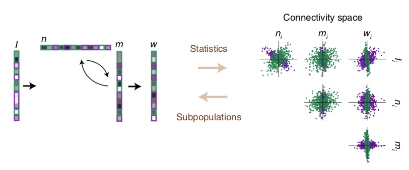
A connectivity space that can be fitted by a mixture of two Gaussians. Two populations (we will call like this each component of the mixture) of neurons are fitted with GMM clustering and colored in purple and green. From (Dubreuil et al. 2022).It turns out that with enough components in the mixture, a rank-$R$ RNN with connectivity parameterized in this way is a universal approximator of $R$-dimensional dynamical systems, so that is theoretically “all we need”! Moreover, the mean-field theory extends naturally to this case, providing explanations of how the different parameters of components of the mixture can be tuned to obtain complex dynamics or modify the network behavior with inputs4. This turns out to be very related to the idea of selective attention via gain modulation: for example a two-population network can implement two tasks by having contextual inputs selectively decrease the gain of the “irrelevant” population in each context. Mean-field theory shows that the “gain” can be decreased without any complex synaptic mechanisms, simply by setting neurons’ activity to the flat part of their non-linear transfer function5.
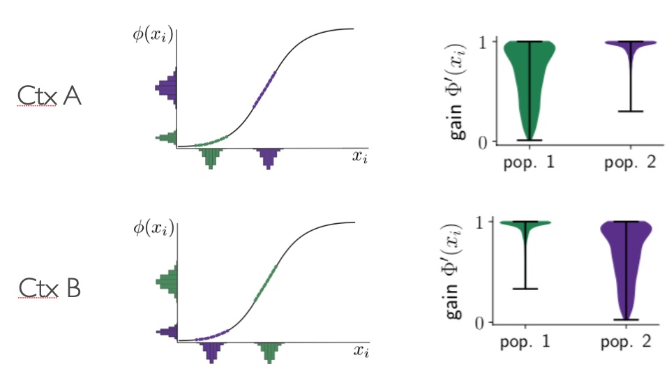
A two-population network can implement two different tasks in two contexts: here histograms of each neurons inputs and firing rates are shown, along with the neural transfer function, for a purple and a green population. In context A, the green population has a lower gain, and only the purple one is performing a task, and it is the opposite in context B. Unpublished figure.The connectivity space gives many more insights into the relation between connectivity and dynamics. For example, by introducing certain symmetries in the connectivity space, we can obtain related symmetries in the dynamics, and implement symmetric attractors like rings and spheres, or polyhedral patterns of fixed points4. And it has probably many more secrets to reveal.
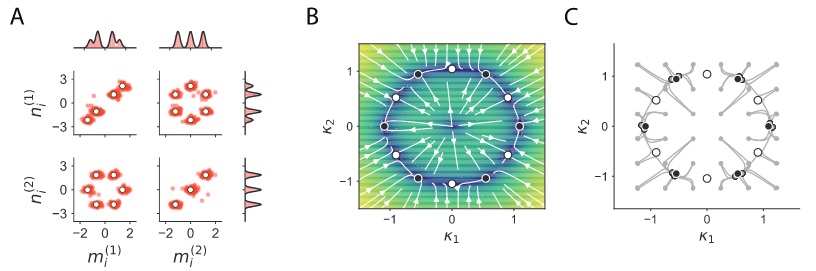
A rank-2 network with 6-fold symmetry in its connectivity space (some projections of it on the left) has a dynamical landscape with similar symmetry, and hence with 6 stable fixed points (black dots in middle and right). From (Beiran et al. 2021a). -
What do low-rank RNNs tell us about “normal” networks?
At this point, you might think that low-rank RNNs are an interesting subject per se, but still be skeptical about their concrete applications to neuroscience or machine learning. Indeed, they are not particularly easy to train, and machine learning people use RNNs that are full-rank for concrete applications. And if you are a neuroscientist, you might have arguments to believe the brain is not a low-rank network: its neurons are spiking and not rate neurons, they have non-symmetric transfer functions, sparse connections, excitatory and inhibitory populations…
Many of these points are being worked out to push low-rank RNNs into the real world, and turn them into practical tools. Let us first tackle the machine learning-side concerns. Do low-rank networks teach us anything about more standard full-rank networks? A first answer is that standard networks have a secret low-rank life! Indeed, when training full-rank networks one can verify that the learned part of their connectivity can be approximated with a matrix that has a very low rank, without any loss of performance6. This shows that low-rank connectivity might arise as a natural solution to computational problems.
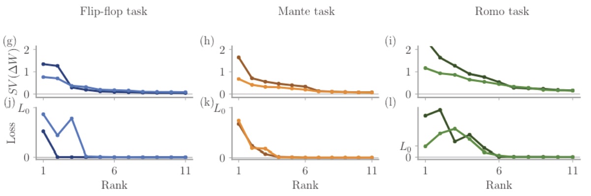
For full-rank networks trained on three different tasks, with two different strengths of initial weight (stronger in lighter colors), the singular values of the learned connectivity (top) as well as the loss when approximating it with matrices of increasing ranks (bottom) are shown. All networks were very well approximated by networks of rank at most 5. From (Schuessler et al. 2020b)
Moreover, ongoing research tends to show that full-rank networks can be reverse-engineered very well by training low-rank RNNs to reproduce their activity (Valente et al in prep).
On the biological side of things, a recently published preprint shows that low-rank RNNs can be made sparse while keeping their properties! Ongoing research shows that positive transfer functions, spiking neurons and Dale’s law can all be added to low-rank RNNs without affecting their computational properties. This is of course to be continued, and there are many more problems to solve if we want the insights of low-rank RNNs to go further in neuroscience, but we hope these results can convince you of their interest in biological modeling.
Summary of low-rank RNNs literature
Here is a quick summary of the research carried on low-rank networks these last few years, hoping you can find the paper that answers your questions:
-
Mastrogiuseppe & Ostojic 20182: in this paper that started the research direction, Francesca and Srdjan introduce the dynamic mean-field theory for low-rank RNNs with a fixed random full-rank noise in the connectivity. They show that these networks exhibit low-dimensional spontaneous dynamics, and they exploit a Gaussian parametrization of connectivity space to build example networks that solve interesting computational neuroscience tasks.
-
Mastrogiuseppe & Ostojic 20197: here, Francesca and Srdjan relate the low-rank framework with reservoir computing, and in particular the FORCE paradigm. In particular, they show how the mean-field theory introduced in the precedent paper can be applied to networks trained on a fixed point task using the least-squares and recursive least-squares methods.
-
Schuessler et al. 2020a4: in (Mastrogiuseppe & Ostojic 2018), the low-rank structure was independent of the fixed random connectivity noise (in a probabilistic sense). Here, Friedrich and his co-authors study the case where the low-rank structure is correlated with the full-rank noise, showing that richer and interesting dynamics arise in this case.
-
Schuessler et al. 2020b6: Friedrich and his co-authors study the dynamics of RNNs trained on a range of cognitive tasks, both experimentally and theoretically. They show that the learned part of the RNN connectivity can be well approximated by a low-rank matrix, and that this phenomenon can be explained by analytical results on low-rank RNNs.
-
Susman, Mastrogiuseppe et al. 20218: Lee, Francesca and co-authors apply a similar paradigm as in (Mastrogiuseppe & Ostojic 2019) to reservoir networks, both open-loop and with a rank-one feedback loop, trained to reproduce a sinusoidal signal. They reveal a “resonance” phenomenon for these networks, analytically deriving a very simple expression for the preferred frequency, and revealing interactions between task and connectivity properties.
-
Beiran et al. 2021a9: Manuel and co-authors extend the Gaussian parametrization of connectivity space to the mixture-of-Gaussians distributions. They show the universality of such networks, and explicit which dynamics can be obtained with a single or with several Gaussian components through a detailed mean-field theory. They also show how symmetries in the connectivity space translate to symmetries in the dynamics of the network, showing in particular how to build networks with symmetric families of attractors.
-
Dubreuil, Valente et al. 20225: Here, Alexis, Adrian and co-authors focus on training low-rank RNNs to do particular tasks and reverse-engineering the obtained solutions. This method reveals that some computational tasks can be accomplished with a single population while others rely on several populations (meaning a mixture with several components in connectivity space, as studied in (Beiran et al. 2021)). In particular, the tasks that require several populations are those that need a flexible input-output mapping, which can be explained through a gain-modulation mechanism.
-
Beiran et al. 2021b10 (preprint): Manuel and co-authors train RNNs to perform flexible timing tasks, both full-rank and low-rank, and study their generalization abilities. These analyses show that low-rank RNNs can generalize better when they rely on tonic inputs, which, as mentioned above, can predictably modify the network dynamics. They also reverse-engineer the low-rank solutions, showing how networks rely on slow manifolds to implement their tasks.
-
Valente et al. 202211: Adrian and co-authors study the relationship between a classical latent dynamics model, the latent LDS (latent linear dynamical system) and linear low-rank RNNs. Although very similar, they are surprisingly technically different. Authors show theoretically and experimentally that they are equivalent when the number of neurons is much higher that the dimensionality of dynamics.
-
Herbert & Ostojic 202212 (preprint): Here, Elizabeth and Srdjan add an element of biological plausibility to low-rank RNNs by showing that they can be made sparser while keeping their interesting properties. Random matrix theory is used to study the effect of sparsity on the eigenspectra of connectivity matrices, and some results of (Mastrogiuseppe & Ostojic 2018) are retrieved with sparse networks.
Notes
-
For an informal introduction through a youtube video, see here. For more formal reviews, see for example Yuste’s historic perspective (Yuste, R. (2015). From the neuron doctrine to neural networks. Nature reviews neuroscience, 16(8), 487-497.) or this more recent review (Vyas, S., Golub, M. D., Sussillo, D., & Shenoy, K. V. (2020). Computation through neural population dynamics. Annual review of neuroscience, 43, 249.). ↩
-
Mastrogiuseppe, F., & Ostojic, S. (2018). Linking connectivity, dynamics, and computations in low-rank recurrent neural networks. Neuron, 99(3), 609-623. ↩ ↩2
-
Notably in the foundational Hopfield networks paper (Hopfield, J. J. (1982). Neural networks and physical systems with emergent collective computational abilities. Proceedings of the national academy of sciences, 79(8), 2554-2558.), but also in position-encoding circuits (Seung, H. S. (1996). How the brain keeps the eyes still. Proceedings of the National Academy of Sciences, 93(23), 13339-13344.) or in learning procedures like FORCE (Sussillo, D., & Abbott, L. F. (2009). Generating coherent patterns of activity from chaotic neural networks. Neuron, 63(4), 544-557.) or the dynamics of gradient descent (Saxe, A. M., McClelland, J. L., & Ganguli, S. (2019). A mathematical theory of semantic development in deep neural networks. Proceedings of the National Academy of Sciences, 116(23), 11537-11546.). ↩
-
Schuessler, F., Dubreuil, A., Mastrogiuseppe, F., Ostojic, S., & Barak, O. (2020). Dynamics of random recurrent networks with correlated low-rank structure. Physical Review Research, 2(1), 013111. ↩ ↩2 ↩3
-
*Dubreuil, A., *Valente, A., Beiran, M., Mastrogiuseppe, F., & Ostojic, S. (2022). The role of population structure in computations through neural dynamics. Nature Neuroscience, in press. ↩ ↩2
-
Schuessler, F., Mastrogiuseppe, F., Dubreuil, A., Ostojic, S., & Barak, O. (2020). The interplay between randomness and structure during learning in RNNs. Advances in neural information processing systems, 33, 13352-13362. ↩ ↩2
-
Mastrogiuseppe, F., & Ostojic, S. (2019). A geometrical analysis of global stability in trained feedback networks. Neural computation, 31(6), 1139-1182. ↩
-
Susman, L., Mastrogiuseppe, F., Brenner, N., & Barak, O. (2021). Quality of internal representation shapes learning performance in feedback neural networks. Physical Review Research, 3(1), 013176. ↩
-
Beiran, M., Dubreuil, A., Valente, A., Mastrogiuseppe, F., & Ostojic, S. (2021). Shaping dynamics with multiple populations in low-rank recurrent networks. Neural computation, 33(6), 1572-1615. ↩
-
Beiran, M., Meirhaeghe, N., Sohn, H., Jazayeri, M., & Ostojic, S. (2021). Parametric control of flexible timing through low-dimensional neural manifolds. bioRxiv. ↩
-
Valente, A., Ostojic, S., & Pillow, J. (2022). Probing the relationship between linear dynamical systems and low-rank recurrent neural network models. Neural Computation, in press. ↩
-
Herbert, E., & Ostojic, S. (2022). The impact of sparsity in low-rank recurrent neural networks. bioRxiv. ↩