RNNs strike back

doi:10.59350/pepzc-the79

Transformers have completely taken by storm the field of sequence modelling with deep networks, becoming the standard for text processing, video, even images. RNNs that were once a very active engineering field have slowly faded into the void. All of them? No, some RNNs are bravely fighting back to claim state-of-the-art results in sequence tasks. The most suprising part? They are linear…

In this post, I want to give a broad introduction for people that do not follow closely the (crazily fast) field of deep learning to the recent developments of sequence modelling, explain why Tranformers have imposed themselves, and why and how RNNs are coming back, as well as describe these new classes of models that are starting to buzz.

Many thanks for help and comments to Nicolas Zucchet.

Table of contents:

• In the previous episodes
• RNNs: the new generation
• Some more tricks
• Are these networks universal learners?
• Intuitively, how do these networks even compute?
• Summary
• Notes

In the previous episodes

We will first recall the precedents, ie. the demise of the RNN and success of the Transformer, and the first apparent limits of the latter. You may skip if you are familiar with Transformers.

Let’s start by the basics. What does a deep network do? It typically aims to model an unknown mapping $f$ from input vectors $x \in \mathbb{R}^N_{in}$ to output vectors $y \in \mathbb{R}^N_{out}$, from a set of datapoints $\{(x_1, y_1), \dots, (x_N, y_N)\}$. In the simplest case, this is done with a multilayer perceptron (MLP) which is simply a series of stacked layers of the form $h^{(k+1)} = \phi\left(W_k h^{(k)}\right)$ with the first $h$ equal to the input and the last to the output. The representational capacity of such models are guaranteed by the universality property that states that for any unknown function $f$ there exists a bunch of parameters $W_1, \dots, W_L$ such that the MLP approximates arbitrarily close the target function (and has actually a fairly simple proof). It doesn’t mean it will be easy to learn, especially depending on the data at hand, but at least the solution does exist. Very well.

But this universality property has its limits within the realm of vectors, of fixed dimension. Most real-world problems, alas, cannot be formulated like this: what if you want to process texts of varying sizes, videos of varying lengths, audios of varying durations? Translate sentences in French to sentences in English, when we don’t even know if the output length will match the input’s? All these problems can fit into a more general formulation though: learning an unknown mapping $f$ from input sequences of vectors $(x_1, \dots, x_T)$ for $T$ taking any value from 0 to infinity, to output sequences $(y_1, \dots, y_{T’})$ with the output length not necessarily equal to $T$. Now, this turns out to be a very general task: it is equivalent to learning an arbitrary program, and as such a system able to learn all such mappings is Turing-complete¹.

But it is not actually so difficult, and it turns out that adding simple non-linear recurrence to the perceptron is sufficient: one can define the vanilla RNN as the system obeying the equations $h_{t+1} = \phi(W_r h_t + W_i x_t)$ and $y_t = W_o h_t$. As simple as it seems, this system has a dynamical universality property: it can approximate as closely as needs be a non-linear dynamical system $y_{t+1} = f(y_t, x_t)$ (again, the proof derives quickly from the perceptron case). This suffices to show that these RNNs are actually Turing-complete, and can hence solve the above problem.

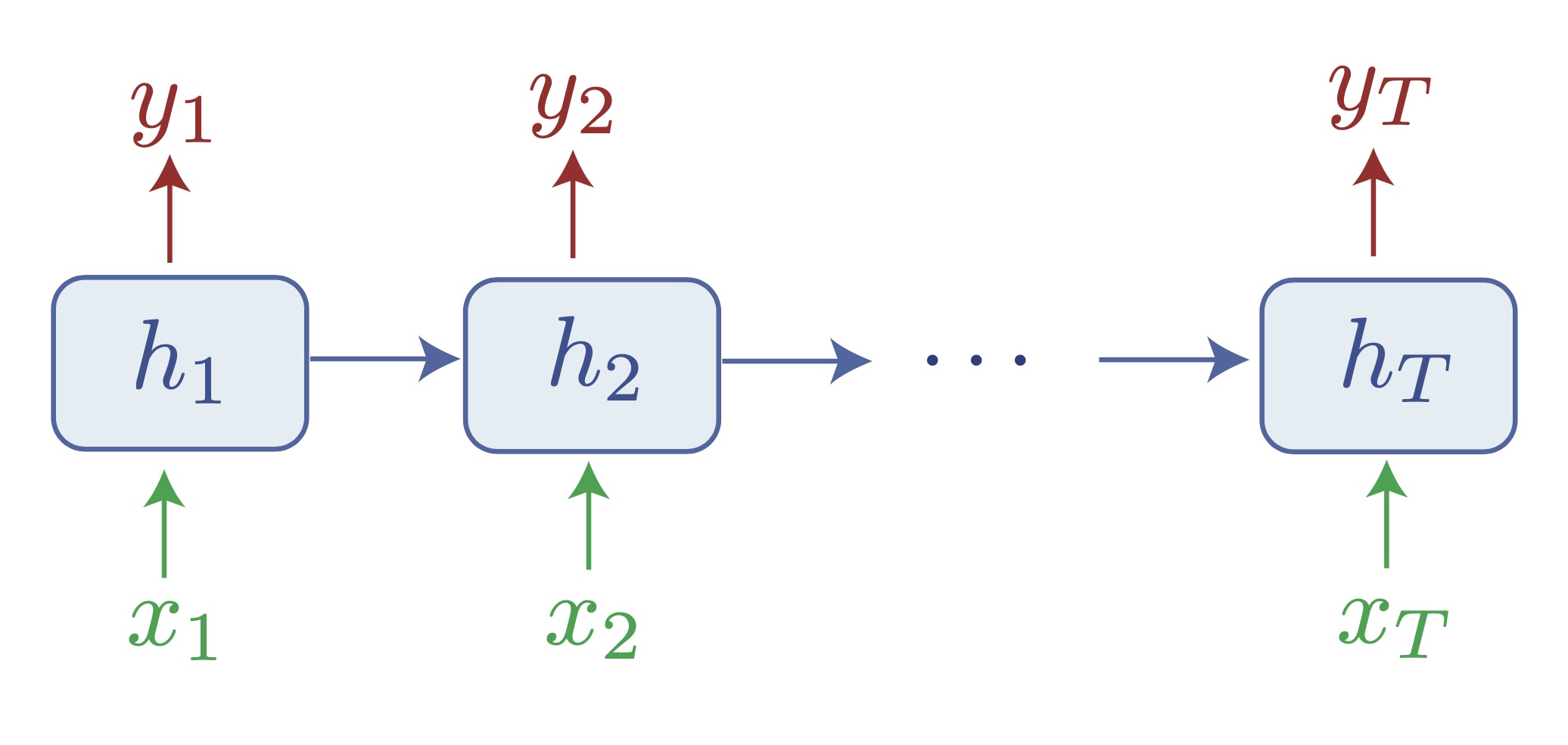
How RNNs aim to solve the sequence-to-sequence learning problem, and approximate any Turing machine. Notice that information travels from one token to another exclusively through the hidden state $h_t$, which effectively acts as a bottleneck.

RNNs with several architectural adaptations (LSTMs, GRUs) have actually ruled the world (or at least language, audio, time series, etc.) for a few years. They have long been very difficult to train, but the literature had slowly progressed to better behaved systems that were able to do basic text classification, language modelling, or translation. Now, they are not even mentioned in the latest textbooks (e.g. Simon Prince’s Understanding Deep Learning). What happened?

Although the above seems like the only obvious solution to learning on sequences, another one exists: what if we processed every vector of the sequence with an MLP? Then we loose all global information about the sequence, not great. Then, what if we authorize this MLP to look at the other elements sometimes, for example through a learned aggregator function $a(x_t, \{x_1, \dots, x_T\})$? This function would be responsible to summarize how the rest of the sequence relates to the element at hand. We could call it “attention”: each $x_t$ would look at the parts of the sequence most relevant to its own information. This is exactly what a Transformer does.

A bird's eye view of the transformer: notice how here tokens "exchange information" via the attention layer, which takes as inputs all tokens (or all preceding tokens if causal masking is active as for a decoder, like GPT). This allows to gracefully handle sequences without dynamics, and avoids the hidden state bottleneck, but without further tricks, notice how this involves quadratic scaling w.r.t the sequence length.

Provided that the function $a()$ can take sequences of any length, we thus end up with a system able to learn mappings on sequences as above, but without the tedious part of having to backpropagate through long iterated dynamics, with all the risks of having vanishing or exploding gradients. Another advantage is parallelization: before, to compute the state of the RNN at timestep $t$, you had to wait until the calculation at the previous timestep was finished. If you wanted to process a sequence of length 1M, this would take minimum 1M clock cycles. Now it can be completely and massively parallelized: if it fits in memory, you can compute at the same time the network layers on all timesteps, just allowing them to share information when needed.

With all this, Transformers really seem like the cool kid. Why would anyone bother with sad RNNs anymore? Well, despite all their properties, Transformers have their dark sides too. First problem, note that $a()$ has to be applied for each element $x_t$ and every time processes the whole sequence. That means that one application of $a()$ does on the order of $T$ computations, and there are $T$ of them to compute $a(x_1, \{x_1, \dots, x_T\})$ until $a(x_T, \{x_1, \dots, x_T\})$. This means to apply attention we actually have to perform $T^2$ computations. Compare to the RNN: we just go through each timestep once, everytime applying a constantly-sized computation, so we get $\mathcal{O}(T)$. First point of the revenge! There are actually a few workarounds to avoid this issue: for example if $a$ is made completely linear, then it there are ways to compute it faster… by actually showing that the computation can be formulated as an RNN²! We will come back to it…

Second issue: in the Transformer as formulated here, each element sees the same series of computations, and hence all information about ordering of elements in the sequence is lost. This information has to be added artifically through another input vector $p_t$ called a positional embedding that can be for example a combination of sine waves of time. The problem is that positional embeddings generalize very poorly out-of-distribution: if a Transformer is trained on sequences of length less than 2000 and tested on longer sequences, even if the architecture and definition of the positional embeddings allow it, performance seems to break. Finding ways around this is a very active area of research, and it is possible that it will not be an issue for very long³, but it is the reason why we so far have fixed (and fairly limited) context windows on all deployed usecases.

Are these mere roadblocks or hard limits for Transformers? Future will tell, but they have already been sufficient to revive interest in RNNs…

RNNs: the new generation

RNNs have always remained an active area of research, but a particular benchmark has been a boon for them: the Long-Range Arena benchmark, released in 2020⁴, combines reasoning and classification tasks over several thousand tokens. The hardest task, Path-X, over 16K tokens, was simply out of the range of any model back then! Suprisingly, all state-of-the-art results on this benchmark have been attained by RNNs⁵. Who are they, and how do they do it?

We will talk here of a small set of influential publications, notably work by the lab of Chris Ré at Stanford and in particular Albert Gu who developed the HiPPO network⁶, then S4⁷, the RWKV indie project⁸ and a more “first-principles” LRU approach by Antonio Orvieto and coauthors⁹. These all seem to rely on very similar principles, and to give a very concrete perspective I will focus on the formalism of the latter publication, although most details will be identical up to minor tweaks, and will hence refer to this module below as an “LRU” (standing for Linear Recurrent Unit).

The fantastic core idea is the following: RNNs are prone to vanishing/exploding gradients because of the non-linearity, and of eigenvalues in the recurrence above 1 (exploding directions) or close to 0 (fast decaying directions). Solution: get rid of both! Which means effectively using linear RNNs. The basic equation of an LRU is thus:

$$ h_t=\Lambda h_{t-1}+B x_t $$

with $\Lambda$ the recurrence matrix, $B$ the input matrix, the $h_t$ are the hidden states and $x_t$ the inputs.

The problem is that linear RNNs are quite boring by themselves: they can only exhibit a fixed point at 0, and then activity that either explodes (eigenvalue > 1), decays to 0 (eigenvalue < 0), stays idle (eigenvalue = 1), or oscillates in clean concentric circles (pair of complex eigenvalues with module = 1). There is some variety but not enough to even get close to the diversity of dynamical systems out there, and all context-dependent operations (for example discovering that “not bad” is positive, not with the valence of “not” and “bad” summed) is out of reach.

We need an additional trick of course, and it consists of adding a non-linear mapping (that will in general be an MLP or even just a Gated Linear Unit function) from the hidden state. Effectively, the output will then be:

$$ y_t = \hat{f}_{\text{out}}(z_t), \text{ with } z_t = Ch_t + Dx_t $$

where $\hat{f}_{\text{out}}$ is the output non-linearity that can be made as complex as one wants, that takes as input a linear readout of the hidden state noted $Ch_t$ (and a skip connection $Dx_t$ that helps without modifying representational capacity). What matters is that all non-linearities are kept above single tokens, they never occur in computations that impact time dynamics of internal states. So dynamics here are always linear.

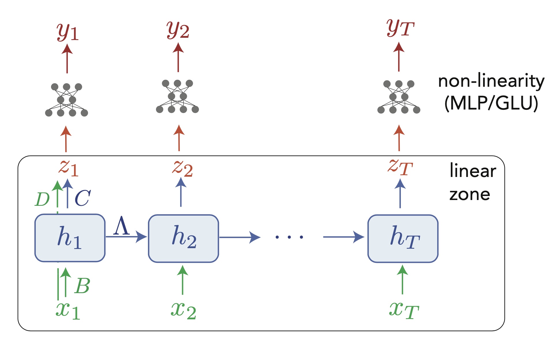
Design of a deep linear recurrence-based network (as in Orvieto et al. 2023). As for a normal RNN, information travels across tokens only through the hidden state $h_t$, that needs to contain all useful informations about the past. Notice that everything below the MLPs involves only linear operations, and the only non-linearities are applied token-wise, above dynamics. Naturally, this architecture can be repeated a few times before reaching the final output. (Notice also the skip connection in the first token, omitted in the next ones for readability.)

That’s all, as simple as it seems! Then stack a few of those one above the other, and you’re good to crush the long-range arena, and even design competitive LLMs! It is astonishing that a system relying only on linear dynamics, supposed to already be boring past the second year of undergrad can reach state-of-the-art results. And they can be made even simpler as we will see below.

In any case, this deserves a few more explanations. If you want more details, in the following, we will cover important tricks, the big universality question (with demo), and some more ideas about these networks.

Some more tricks

• Recurrence was already linear, if that is not simple enough, you can just make it diagonal. Effectively, this means in the equations above that we can parametrize $\Lambda = \operatorname{diag}(\lambda_1, \dots, \lambda_d)$, with the important caveat that the $\lambda_i$ are complex numbers. Effectively, this means that all tensors in the computation graph will be complex numbers, which torch and jax handle pretty well with gradients. Even accounting for the fact that eigenvectors can be pushed to the input and output matrices of the recurrence ($B$ and $C$), it remains a suprising fact (for the linear algebra nerds, it means that the nilpotent components in the Dunford reduction of $\Lambda$ can be thrown away). References about this fact are this paper by Gupta et al¹⁰. and the Orvieto et al.⁹ too.

• As you may know, linear recurrences have four possible behaviors depending on each complex eigenvalue: divergence to infinity ($|\lambda| > 1$), convergence to fixed point ($|\lambda| < 1$), line attractor ($\lambda = 1$), and oscillatory mode ($|\lambda| = 1$ and $\lambda \neq 1$). We obviously want to avoid divergence to infinity that will crash our program, so we need to restrict the $\lambda_i$ to always have a module smaller than 1. For the rest, we may be interested in decaying modes, that allow to forget some information after some time, but if the goal is to keep as much information stored for as long as possible, this should also be avoided. That means that for the most part, the $\lambda_i$ should have modules close to 1. This will also allow gradients to flow further in time. A clean parametrization proposed in Orvieto et al. to enforce this characteristic is:
  $$ \lambda_i = \exp(-\exp(\nu_i) + i\theta_i) $$

  where $i$ is the imaginary number, and hence the module equal to $\exp(-\exp(\nu))$ is necessarily smaller than 1! This is called the exponential parametrization, and people have noticed it considerably facilitated training.

• Linear RNNs can be parallelized across timesteps too! Remember that a major motivation for Transformers was the possibility to compute in parallel outputs for several tokens, something that is impossible for RNNs since one has to go through states one after the other. It turns out that by making an RNN linear, parallelization becomes possible. Indeed, the value of the hidden state at any timesteps can be computed analytically through a simple formula:
  $$ h_t = \sum_{k=0}^t \Lambda^k B x_{t-k} + \Lambda^t h_0 $$

  this can be seen as a convolution of sorts on the inputs $x_k$. This was actually one of the big motivations for getting rid of the non-linearity in recurrence only, and leads to a fast algorithm described in detail in section 2.4 of the S4 paper⁷. Note the goal is not to compute all tokens in parallel, we would get the same quadratic explosion as for Transformers past a point, but to parallelize recurrence by chunks to better use tensor-handling capabilities of GPUs. Also note that for diagonal $\Lambda$, computing the matrix powers means simply exponentiating the $\lambda_i$, so again, everything falls together nicely!

• A lot of additional details are in the papers, notably the idea that one needs to initialize the $\lambda_i$ particularly close to a module of 1, take into account their phase, and many other things that improve training.

Are these networks universal learners?

Now for the big question: our system so far is essentially a simple linear DS followed by a token-wise non-linearity. Is this a universal approximator of dynamical systems, and a Turing-complete system just as the vanilla RNN? This idea seemed crazy at first, given the limited nature of linear dynamics, but we can just test it! I ran some tests with a one-layer LRU network (with three-layer MLP as its output), parametrized as above, and trained it to do some simple but very non-linear things, like reproduce a bistable, double-well 1D system¹¹. After some tinkering, here are some quick results:

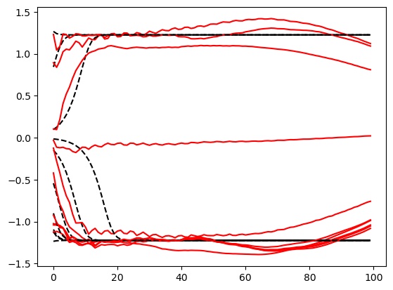
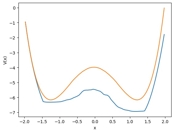
Left: Some target (black) and network-produced (red) trajectories. Right: 1D potential of the target double-well DS (orange) and that obtained by the fitted network (blue).

There is no doubt that the LRU manages to capture intrinsically non-linear dynamics with its little linear engine. Understanding how this kind of phenomena arise exactly will be an interesting research project for the future, as well as proving mathematically what the exact capabilities and limits of such networks (a recent proof of universality for example in this preprint¹²). Here’s a quick intuition: we aim to reproduce unknown dynamcis $y_{t+1} = f(y_t, x_t)$ with a system such that $y_t = g(h_t)$ and $h_{t+1} = Ah_t + Bx_t$, by learning a universal mapping $g$, and matrices $A$ and $B$. Let us assume that for any sequence $x_1,\dots, x_T$ we can guarantee that the sequences $h_1,\dots,h_T$ will be always different, and we won’t get the same $h_i$ for two different input sequences. Then it becomes trivial to just learn a $g$ such that for a given $y$, for any $h$ that will be in the precursor set $g^{-1}(y)$, then $g(Ah + Bx) = f(y, x)$. Our assumption though is not trivial, but by keeping $T$ fixed and increasing the hidden dimensionality $N$ we can always achieve it, an example solution being a block-circulant matrix such that $A^T = Id$ and such that all $A^tB$ have orthogonal column spaces. This requires $N = T \times N_{in}$ obviously.

Addendum: I thought any approximations results of the style would only hold on finite time intervals, but I was pointed to a fantastic proof by Stephen Boyd and Leon Chua¹³ showing approximations of non-linear dynamics with a linear DS can actually hold in infinite time intervals, provided that they have a property called fading memory which is exactly what one would think it is: differences of inputs in the far past have decreasing influence on present state (so not chaotic). However… If you care about long-term dependencies, till what point do you want the fading memory property to hold? #foodforthought

Addendum 2: At this point I think it is essential to add a few words about this “HiPPO” theory I mentioned along the way, because it is a very beautiful and slightly orthogonal view of the problem. The idea behind the design of S4 and its precursor⁶ is to summarize as well as possible the input sequence into the final hidden state. We know ways to efficiently summarize sequences or signals in an Euclidean representation, for example through Fourier series or the less known Legendre polynomials. Early works have proposed recurrent units that computed Fourier¹⁴ or Legendre¹⁵ coefficients of an input signal in an online fashion, but the general framework was formalized in Albert Gu’s “High-order Polynomial Projection Operators” work that forms the basis for all these developments⁶. It requires quite a bit of maths, but it also makes one of the most grounded frameworks in DL.

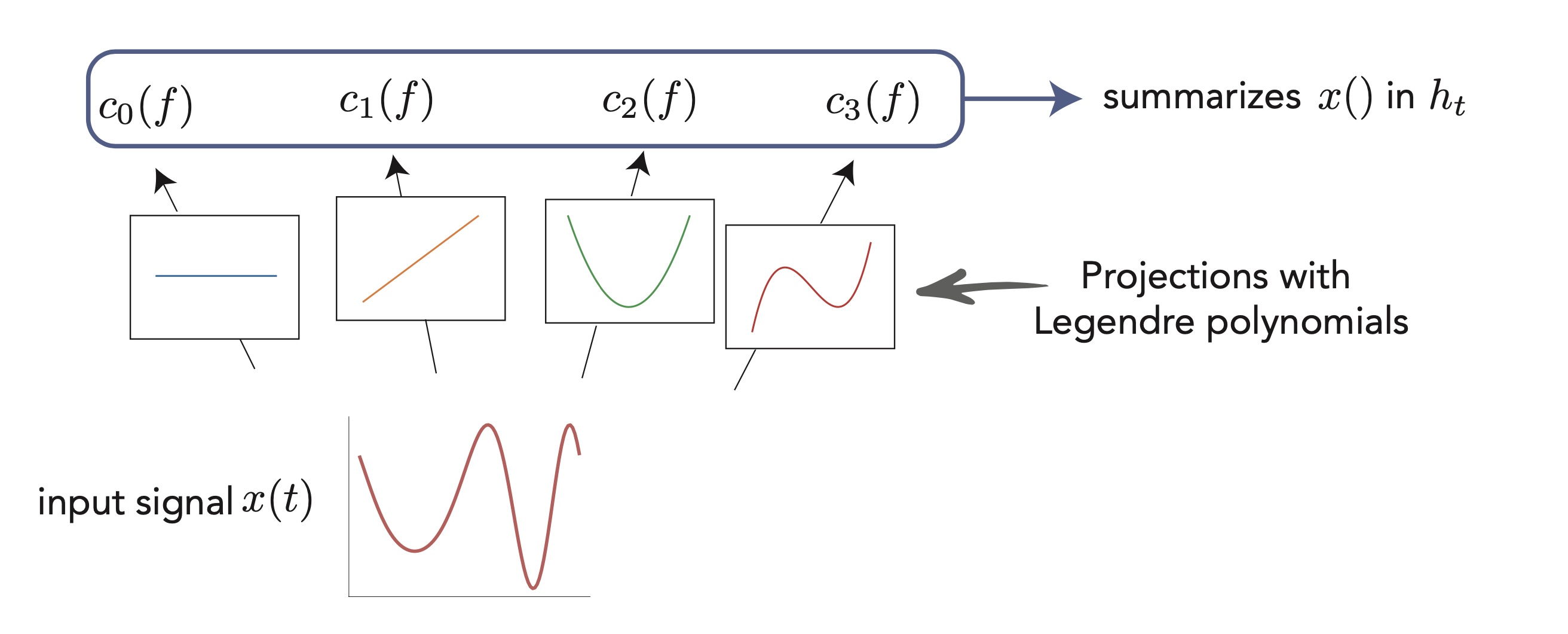
Another view of linear recurrent networks through the HiPPO lens: consider that you have a input "signal" (here a continuous $x(t)$, but it could be a sequence of $x_t$), and you want to "summarize" it in the last hidden state $h_t$. The idea is to project this signal on a appropriate basis of functions, like cosines and sines of increasing frequencies (Fourier basis), or as illustrated here the set of Legendre polynomials. This gives a set of coefficients that we may want to see in the last hidden state. The HiPPO works provides a mathematical framework to do this online (ie. updating as the inputs arrive) with a linear RNN!

In fact it is fascinating to see that given enough memory space a linear DS can accomplish all sorts of interesting things. A paper by Zucchet, Kobayashi, Akram and colleagues¹⁶ for example shows how they can reproduce a Transformer-like attention mechanism. Theoretical constructions always require capacities that would preclude any advantages of such networks, but in practice they seem to get along pretty well. In the end, how do they compute?

Intuitively, how do these networks even compute?

One thing that is particularly striking now is that these networks seem to have a fundamentally very different nature than traditional non-linear RNNs. The former ones are believed to compute mostly by exploiting interesting dynamical structures, like fixed points¹⁷, more fancy topological shapes like rings, spheres and toroids, and rich non-normal transients. None of this is possible with LRUs. Their only possibility is to throw inputs into a large bunch of slowly oscillating modes, and then learn useful patterns from these internal rich melodies. As a weird analogy, it reminds me of the concept of epicyclic computing by which Ptolemeus was able to fit very complex astronomical motions using carefully adjusted sets of numerous rotating gears. Similarly, it might be that by having enough oscillating modes of diverse frequencies and phases, LRUs are epicyclic computers able to generate useful patterns from data, through which non-linear dynamics are ultimately learned.

A quick demonstration of the phenomenon is the following: in one of the papers cited above¹⁷, RNNs were trained to perform the “flip-flop task”, which consists in receiving upwards or downwards pulses and keeping in memory the direction of the last pulse received. Very striking dynamical landscapes appeared when dissecting these RNNs, with notably fixed point attractors that encoded the memory of last pulse received. An LRU net can perfectly be trained to do this task, as demonstrated below, but this time no internal bistable attractors are to be found, and recurrent units simply keep oscillating, as they should do.

Experiment on memory without attractors: left: output (blue) and input (blue) of a network trained to do the flip-flop task. Right: activity of some recurrent units of this network (more precisely between recurrent and matrix and non-linearity). They exhibit indeed a mix of fading and oscillating activity, but no sustained attractors.

I cannot close without strongly advising a recent paper by Il Memming Park’s group¹⁸ which demonstrates continuous attractor-like behavior without internal dynamical attractors, and with oscillating dynamical modes instead, and outlines a rich theory. All this points, I think, to a deep dichotomy between two different ways of computing with high-d dynamics, and advantages and disadvantages of each will be interesting to understand, as well as figuring out which one brains are using.

Summary

• The recent class of linear recurrent networks, which comprises works such as H3, S4, S5, RWKV and the LRU notably are simply composed of linear RNNs stacked with token-wise non-linear MLPs.
• Even though their internal dynamics are linear, they are able to fit all sorts of non-linear dynamics.
• They are successful because they address several shortcomings of Transformers (quadratic explosion, positional encoding) that become critical for long sequence tasks.
• Their precise theoretical limits remain to be fully assessed, but with a number of neurons scaling up with the number of timesteps they do have some form of universality.
• At the core, they seem to rely on a fundamentally different paradigm than classical RNNs: instead of relying on attractors they use oscillatory modes, throwing their inputs into a maelstrom of rotations from which the feedfoward MLPs are tasked to extract meaning.
• Having a new recurrent computation paradigm is exciting, and promises lively future debates, for example about the role of linearity in the brain.

Notes

1. Kenji Doya, Universality of fully-connected recurrent neural networks, 1993 ↩

2. Katharopoulos et al., Transformers are RNNs: Fast Autoregressive Transformers with Linear Attention, 2020 ↩

3. See this write-up: https://kaiokendev.github.io/context ↩

4. Tay et al., Long Range Arena: A Benchmark for Efficient Transformers, 2020 ↩

5. Benchmark results ↩

6. Gu, Dao et al., HiPPO: Recurrent Memory with Optimal Polynomial Projections, 2020 ↩ ↩² ↩³

7. Gu et al., Efficiently Modeling Long Sequences with Structured State Spaces, 2021 ↩ ↩²

8. RWKV project, Peng et al., RWKV: Reinventing RNNs for the Transformer Era, 2023 ↩

9. Orvieto et al., Resurrecting Recurrent Neural Networks for Long Sequences, 2023 ↩ ↩²

10. Gupta et al., Diagonal State Spaces are as Effective as Structured State Spaces, 2022 ↩

11. Network trained to reproduce at its outputs trajectories sampled from the target DS with random initial points, and additionally an MLP encoder that maps from the initial state to an initial $h_0$ for the LRU. ↩

12. Orvieto et al., On the Universality of Linear Recurrences Followed by Nonlinear Projections, 2023. My understanding is that the proof involves showing that there can be a bijection from input sequence to final hidden state if N is large enough, but I’ll have to read it again. ↩

13. Boyd & Chua, Fading Memory and the Problem of Approximating Nonlinear Operators with Volterra Series, 1985 ↩

14. Zhang et al., Learning Long Term Dependencies via Fourier Recurrent Units, 2018 ↩

15. Voelker et al., Legendre Memory Units: Continuous-Time Representation in Recurrent Neural Networks, 2019 ↩

16. Zucchet, Kobayashi, Akram et al. Gated recurrent neural networks discover attention, 2023 ↩

17. Sussillo and Barak, Opening the Black Box: Low-Dimensional Dynamics in High-Dimensional Recurrent Neural Networks, 2012 ↩ ↩²

18. Park et al., Persistent learning signals and working memory without continuous attractors, 2023 ↩