When I try to avoid working on my doctoral projects, I like to get lost in the statistical world, to marvel at the seemingly infinite amount of statistical methods out there, and think how they are all related and yet different. There is one particular tool that I have recently seen in many different studies in neuroscience and has caught my attention: Canonical Correlation Analysis, or CCA for friends. It has been used for example to find activity shared accross multiple brain areas (Semedo et al 2019), to align neural recordings done in different days (Gallego & Perich et al 2020), or to verify if multiple neural networks use similar representations (Kornblith et al 2019) or mechanisms (Maheswaranathan & Williams 2019). How can a method appear in so many different context? In this post, I will introduce this hidden child of PCA and Pearson’s correlation, try to give insights on what it exactly does, and touch on some of its pitfalls.

What CCA solves

To understand a tool, I like to understand the problem it solves, and CCA is already peculiar from this point of view, since one can come at it as the answer to many different questions (actually 3 big ones).

Multivariate correlation

Let us first consider the question of correlation. When one has two scalar variables in a dataset, $\{x_i\}$ and $\{y_i\}$, for example vaccination status and hospitalization status, it is easy to check if they are related by computing their Pearson correlation coefficient given by :

$$ r = \frac{\sum_i (x_i - \overline{x}) (y_i - \overline{y})}{\sqrt{\sum_i (x_i - \overline{x})^2 \sum_i (y_i - \overline{y})^2}} $$

(with $\overline{x}$ and $\overline{y}$ representing the means of $x$ and $y$). Everybody knows of course this is a dangerous tool that should be used with extreme care, but it is also unavoidable in science, and a good first step in exploring datasets.

Now, let us say one wants to compare not two scalar random variables, but two random vectors in a dataset, $\{\mathbf{x}_i\}$ and $\{\mathbf{y}_i\}$. Sometimes the coordinates of those vectors have a definite role and can be matched. For example if you are comparing the multivariate scores on some psychological test of a parent and its child, it makes sense to compute a correlation for each coordinate of the test, and then consider an average correlation. This is also a good solution when one wants to verify the fit of a model to some experimental, when each variable of the model is specifically targeted at modelling one of the measured variables.

But as one moves towards more complex models that representing the interaction of many simple entities, like a neural network is, one may lose track of individual variables when trying to capture global behavior. For example, let us say we have an artificial neural network model that we want to match to a neural recording. A first solution to tackle this problem is to match each neuron of the recording to one “best-fitting” neuron in the model, like is done in most of Yamins and DiCarlo’s works. This solutions needs extreme care to avoid weird statistical biases. It would be nice to have a number like the $r$ correlation coefficient that summarizes the “similarity” of unaligned data.

One way to look at it is by thinking of two shapes in 3D spaces that are not necessarily aligned. It would be nice to have a summary value that can tell how similar the shapes are when they are “as aligned as possible”. That is exactly what CCA does. But before explaining how, let’s come at it from another perspective.

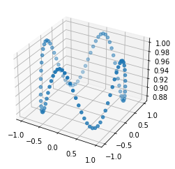
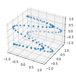
Figure 1: these 2 things look quite similar, but how to measure this if they aren't even aligned?

“Crossed” PCA and alignment

Let us again consider the problem of the 2 shapes in 3D, but this time consider the two shapes in figure 2 : if you look at the points from above, they look exactly the same, but when looking from the side, you see how they are different : the depth value of the points is all scrambled. A two-dimensional being looking at these shapes from random perspectives might be interested in a method telling him that they look identical when seen from above. This is exactly the problem that CCA solves : it finds directions where the two sets of vectors are maximally correlated. From this perspective one can understand it either as a dimensionality reduction method, telling you which projections of the data to look at to find most correlation, or as an alignment. It is also obvious how this is related to our first question : by aligning the shapes first axis by axis, it is then direct to compute their correlation.

Figure 2: 2 shapes that look very similar from the top, but actually aren't that much.

To summarize, CCA can be seen as three things :

a multivariate extension of Pearson’s correlation coefficient
a dimensionality reduction method finding subspaces where two sets of vectors look very correlated
an alignment tool (kind of like Procrustes’ analysis I guess)

NB: for the alignment purpose, it is important to note that it works for datasets that are matched (ie. each sample $\mathbf{x}_i$ corresponds to exactly one sample $\mathbf{y}_i$. If they aren’t matched, and are just two a priori unrelated point clouds, one has to look at Procrustes’ analysis instead).

How it works

As we mentioned, CCA takes as input two linked sets of vectors $\{x_i\}$ and $\{\mathbf{y}_i\}$, with the $\mathbf{x}$’s and $\mathbf{y}$’s of two not necessarily equal dimensionalities $d_1$ and $d_2$. We can put them into two data matrices $\mathbf{X} \in \mathbb{R}^{N \times d_1}$ and $\mathbf{Y} \in \mathbb{R}^{N \times d_2}$. Note that contrarily to the dimensionality, the number of samples $N$ has to be equal accross the two datasets (as is the case for Pearson’s correlation coefficient as well). Also note in everything that follows I will considered data has been centered (mean of $\mathbf{x}$ and $\mathbf{y}$ is 0 on each coordinate).

The goal of the method is to first find a direction $\mathbf{a}_1 \in \mathbf{R}^{d_1}$ and a direction $\mathbf{b}_1 \in \mathbb{R}^{d_2}$ such that $\mathbf{X}$ and $\mathbf{Y}$ projected on these directions are maximally aligned, ie. such that :

$$ \mathbf{a}_1, \mathbf{b}_1 = \operatorname{argmax}_{\mathbf{a}, \mathbf{b}} \operatorname{Pearson}(\mathbf{X}\mathbf{a}, \mathbf{Y}\mathbf{b}) $$

Once we found this first direction, we may wish to repeat the process with the rest of the data, ie. $\mathbf{X}$ projected on the orthogonal subspace of $\mathbf{a}_1$ and $\mathbf{Y}$ projected on the orthogonal of $\mathbf{b}_1$. This will give two new directions, on which the correlation will be equal or less than the first one, and so on until we obtain $m$ pairs of directions, on which the two datasets are progressively less and less correlated.

In the end, CCA’s output is quite similar to PCA’s: we get two orthogonal matrices $\mathbf{A}$ and $\mathbf{B}$, of respective shapes $d_1 \times m$ and $d_2 \times m$ where $m = \operatorname{min}{d_1, d_2}$, which map the original datasets $\mathbf{X}$ and $\mathbf{Y}$ to a common subspace where they are maximally aligned, by the transformations $\mathbf{X}\mathbf{A}$ and $\mathbf{Y}\mathbf{B}$. We also obtain a series of $m$ numbers $1 \geq \rho_1 > \dots > \rho_m \geq 0$ which correspond to the decreasing correlation coefficients of each of the aligned directions: $\rho_i = \operatorname{Pearson}(\mathbf{X}\mathbf{a}_i, \mathbf{Y}\mathbf{b}_i)$.

The easiest way to make CCA work is to install the excellent statsmodels library for python, and to use its class CanCorr. A few lines of code will be more telling :

from statsmodels.multivariate.cancorr import CanCorr
cc = CanCorr(X, Y)  # where X and Y and two numpy arrays, of shapes nxd1 and nxd2
A = cc.y_cancoef
B = cc.x_cancoef
X_al = X @ A
Y_al = Y @ B
print(cc.cancorr)  # these are the ordered canonical correlations

That way, CCA performs its role as a dimensionality reduction and alignment tool. A summary similarity statistic between the two datasets can easily be obtained by taking for example the average of the canonical correlations, but it is of course more telling to keep the whole distribution of these correlations.

The algorithm

If you wish more details about how the algorithm works, you can find two very nicely explained derivations here. I cannot do any better than this report, so I will try to give some personal thoughts about how to interpret this algorithm

I am going to look at the SVD implementation to get some insights. Briefly, the algorithm takes the SVD of each dataset:

$$ \mathbf{X} = \mathbf{U}_1\mathbf{S}_1\mathbf{V}_1^T \\ \mathbf{Y} = \mathbf{U}_2\mathbf{S}_2\mathbf{V}_2^T $$

Then takes the SVD of the matrix $\mathbf{U}_1^T\mathbf{U}_2$:

$$ \mathbf{U}_1\mathbf{U}_2^T = \mathbf{U}\mathbf{S}\mathbf{V}^T $$

and finally $\mathbf{S}$ here contains the canonical correlations while $\mathbf{A} = \mathbf{V}_1\mathbf{S}_1^{-1}\mathbf{U}$ and $\mathbf{B} = \mathbf{V}_2\mathbf{S}_2^{-1}\mathbf{V}$. This looks awfully complicated, but it actually makes a lot of sense. Let me explain.

The way PCA typically works is by considering the diagonalization, which happens to also be the SVD, of the covariance matrix of some data : $\mathbf{X}^T\mathbf{X} = \mathbf{U}\mathbf{S}\mathbf{U}^T$. When looking at two datasets, it seems natural to do an SVD on the covariance $\mathbf{X}^T\mathbf{Y}$. This can perfectly be done and will give some insights, but the problem is it mixes internal variance of the datasets with their correlations: if one axis of $\mathbf{X}$ has a huge variance compared to the others, it will dominate the SVD of the covariance, even if it is not so correlated with any of the directions in $\mathbf{Y}$.

The most reasonable workaround is to start by “whitening” each dataset, that is applying a linear transform so that (i) each coordinate of the data is independent of the others (orthogonality) and (ii) each coordinate of the data has a variance of 1 (normalization). Multiplying by $\mathbf{V}_1\mathbf{S}_1^{-1}$ corresponds exactly to those two steps, so that $\mathbf{U}_1$ and $\mathbf{U}_2$ are simply the whitened versions of $\mathbf{X}$ and $\mathbf{Y}$. It then suffices to apply the SVD to the covariance matrix of these two matrices to obtained canonical correlations (and one can show that those singular values will be contained between 0 and 1). Finally, $\mathbf{A}$ simply works by applying first the whitening transform, and then transforming into the left canonical basis found by the covariance SVD, and similarly for $\mathbf{B}$. This whitening step is actually very similar to the notion that Pearson’s correlation is simply the covariance of whitened data, as explained in my previous post.

I have to admit however that I am still not convinced that this whitening step is always desirable when we are comparing datasets, and I would say it is still useful to keep the “SVD on covariance” algorithm in mind when treating data. The amazing Kornblith paper I mentioned in the introduction actually tackles part of this question: in their framework, the “SVD on covariance” algorithm is called Linear CKA (Centered Kernel Alignment), and avoids some pitfalls, one of which I will mention in the next paragraph.

CCA’s traps

As any good statistical methods, there is probably a million ways CCA can be misused. I noticed one while I was using it with high dimensional data, that I will illustrate here: take two perfectly random matrices $\mathbf{X}$ and $\mathbf{Y}$ of increasing dimensionality, as in the code below, and you will observe something similar to figure 3.

N = 2000
fig, ax = plt.subplots(1, 3, figsize=(12, 4))

for i, d in enumerate((50, 200, 1000)):
    X1 = np.random.randn(N, d)
    X2 = np.random.randn(N, d)
    cc = CanCorr(X1, X2)
    ax[i].bar(x=np.arange(d) + 1, height=cc.cancorr, width=1.)
    ax[i].set_ylim(0, 1)
    ax[i].set_xlabel('component')
    ax[i].set_xlabel('can. corr.')
    ax[i].set_title(f'd={d}')

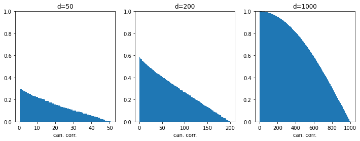
Figure 3 : A curse of dimensionality: catastrophic increase of top canonical correlations.

As we can see, when the data becomes very high dimensional, the highest canonical correlations will become as high as 1, probably because it becomes likely that among all these possible dimensions the algorithm will find some that match well between the two datasets (like you would easily find two people with the same birthday in a big enough group).

The simple workaround for this issue is simply to apply a first step of PCA to each of the datasets, forming $\tilde{\mathbf{X}}$ and $\tilde{\mathbf{Y}}$ by keeping only the first $m$ principal components of $\mathbf{X}$ and $\mathbf{Y}$, where $m$ is reasonably small number chosen by the user. This will keep the “main signal” part of the data, as it is likely that for very high dimensional data most of the dimensions simply contain noise anyway. With the 1000-dimensional datasets of above, choosing $m=10$ for example brings canonical correlations to the expected null values. This method is then called SVCCA, and summarized in a nice paper (Raghu et al. 2017).

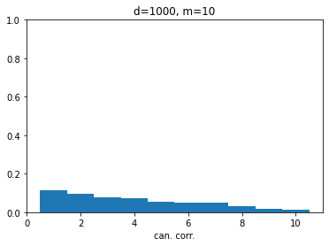
Figure 4 : With singular values, we are saved!

Globally however, since the algorithm maximizes its objective, it seems reasonable to think that it will always overestimate the real underlying correlations (a classic case of maximization bias). Mmh… Keep safe when doing stats everyone!

Biblio

(Gallego & Perich et al 2020): Long-term stability of cortical population dynamics underlying consistent behavior, Nature Neuroscience, 2019

(Kornblith et al 2019): Similarity of Neural Network Representations Revisited, ICML 2019

(Maheswaranathan & Williams 2019): Universality and individuality in neural dynamics across large populations of recurrent networks, NeurIPS 2019

(Raghu et al. 2017): SVCCA: Singular vector canonical correlation analysis for deep learning dynamics and interpretability, NIPS 2017

(Semedo et al 2019): Cortical Areas Interact through a Communication Subspace, Neuron, 2019